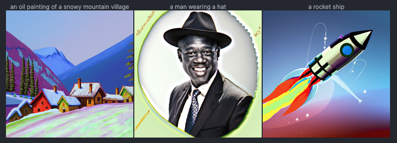
50 Inference Steps
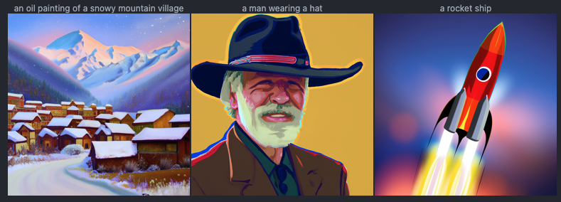
20 Inference Steps
In this project, I experimented with pre-trained diffusion models, implemented sampling loops, and used diffusion models for inpainting and creating optical illusions.
Using pre-computed Text Embeddings, I generated images using the following captions with the DeepFloyd IF model. I used random seed 12345 for the generations. The model's generations are quite good and adhere very well to what the prompt said which were added given their pre-computed text embeddings.

50 Inference Steps

20 Inference Steps
To get a noisy image, the sampling noise loop was implemented using the following equations, which scale and add noise to an image.


Original Image

Noise t=250

Noise t=500

Noise t=750
An attempt to denoise the images with gaussian blur filtering is shown, however, the results are quite poor, which is why more complex methods are necessary.

Noise t=250

Noise t=500

Noise t=750

Denoise t=250

Denoise t=500

Denoise t=750
Given the pre-trained DeepFloyd model, one-step denoising was attempted by estimating the noise from the model given the timestamp, and getting the original image by solving the noise equation for x0. For noise closer to 0, the one-step denoising is better, but images closer to T=1000, the model does much worse. Even though DeepFloyd is trained on an extremely large dataset of x_t and x_0 pairs, one step denoising is not enough to generate high quality images.

Noise t=250

Noise t=500

Noise t=750

One-step Denoise t=250

One-step Denoise t=500

One-step Denoise t=750
Now, the denoising is done iteratively, rather than in one step, from the noisy image to t=0, a clean image. This is done by following equations 6 and 7 from the DDPM Paper. However, because iteratively denoising from t=1000 all the way to 0 requires too much compute, the process is streamlined by striding the timesteps by a factor of 30, starting from 990 and going down to 0. The iterative method interpolates between the estimated clean image and noise, and takes the output from the noiser timestep, and iteratively denoises it until the time reaches 0. The prompt is specified as "a high quality photo", essentially representing a null prompt. The denoising is also started at timestep 690, rather than 1000, to try and help recreate the image rather than generate a random one.


Original

Iteratively Denoised

One-step Denoised

Gaussian Blurred

t=690

t=540

t=390

t=240

t=90
Now, images are generated from scratch by starting with random noise and starting with i_start=0 so that the timestep starts at the max and goes down to 0. Here are 5 images generated with the prompt as "a high quality photo".


To improve image quality, while losing some image diversity, guidance is introduced. This is done by introducing an unconditional noise estimate, which is the model's prediction of noise with a true null text prompt and changing the actual noise estimate to follow the follow equation, where the gamma is set to 7. In this case, if gamma is 0, the noise estimate is simply the unconditional prediction, if it is 1 it is only the conditional, but when it is greater than 1, guidence is introduced.


Image-to-Image translation can be done by putting the image through the noise schedule, but changing the initial noise step that denoising is started from. The closer denoising starts to the original image, the more similar it will be to the original image which is noised. Denoising is done with the iterative CFG method.

i_start = 1

i_start = 3

i_start = 5

i_start = 7

i_start = 10

i_start = 20

Campanile
Using the same process as above, image editing of both images from online and images hand-drawn can be done.

i_start = 1

i_start = 3

i_start = 5

i_start = 7

i_start = 10

i_start = 20

Web Image 1

i_start = 1

i_start = 3

i_start = 5

i_start = 7

i_start = 10

i_start = 20

Web Image 2

i_start = 1

i_start = 3

i_start = 5

i_start = 7

i_start = 10

i_start = 20

Hand Drawn Image
Image inpainting can be performed by using a mask and denoising a random noise sample within the mask. First, denoise the entire image, and then set everything outisde of the mask to be the original image with the noise schedule at that given time step.


Campanile

Mask

Replace

Inpainted

Big Ben

Mask

Replace

Inpainted

Amalfi Coast

Mask

Replace

Inpainted
Using the same process as the previous image-to-image translation, the conditional denoising can be based on a specific text prompt, rather than a general prompt. This conditioning was based on "A rocket ship".

i_start = 1

i_start = 3

i_start = 5

i_start = 7

i_start = 10

i_start = 20

Campanile
With the pre-trained diffusion model, Visual Anagrams can be implemented by using two different conditional text prompts and averaging the flipped noise estimate for one. Each row is the same image where the image on the right is the left image flipped.
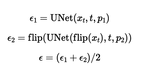

An oil painting of people around a campfire

An oil painting of an old man

An oil painting of a snowy mountain village

A man wearing a hat

A photo of a hipster barista

A man wearing a hat
Using a similar idea as the visual anagrams, hybrid images can be generated which will seem like a photo of something from close up, but something different from further away. This is done by following the algorithm below with high and low pass filters
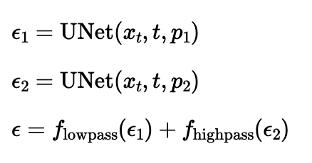

Hybrid image of a skull and waterfall

Hybrid image of waterfall and a man

Hybrid image of a snowy mountain village and dog
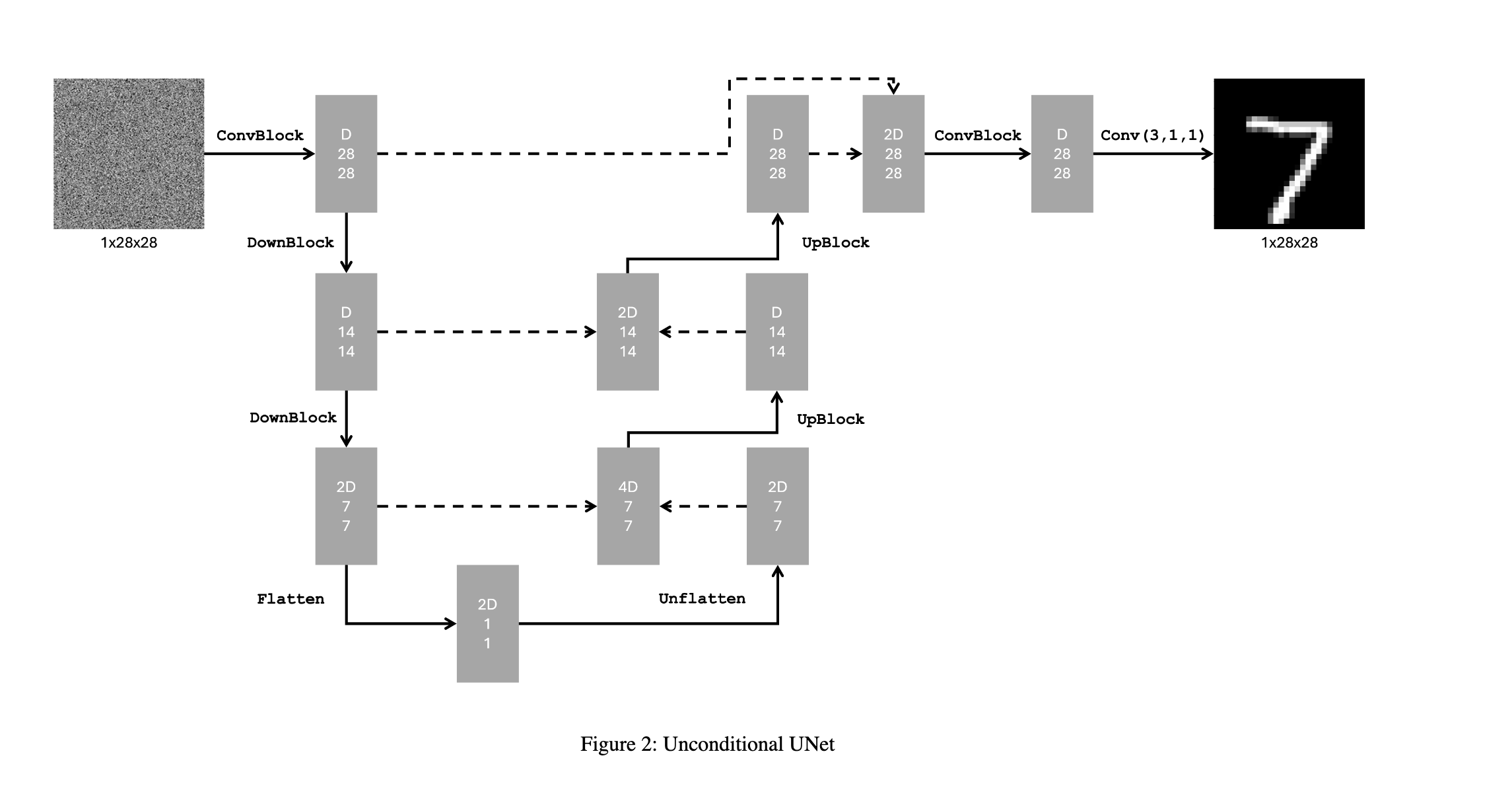
First, I implemented an unconditional U-Net based on the following architecture to denoise data in a single step.
Dataset along with various sigma values for adding noise to the image.

sigma = 0.0

sigma = 0.2

sigma = 0.4

sigma = 0.6

sigma = 0.8

sigma = 0.0

sigma = 0.2

sigma = 0.4

sigma = 0.6

sigma = 0.8

sigma = 0.0

sigma = 0.2

sigma = 0.4

sigma = 0.6

sigma = 0.8

sigma = 0.0

sigma = 0.2

sigma = 0.4

sigma = 0.6

sigma = 0.8
The hyperparameters for training the model are as follows:
Here are the model results on the test set after the first and last epochs at varying sigma values for image noise.
After Epoch 1

sigma = 0.0

sigma = 0.2

sigma = 0.4

sigma = 0.6

sigma = 0.8

sigma = 1.0

Output

Output

Output

Output

Output

Output
After Epoch 5

sigma = 0.0

sigma = 0.2

sigma = 0.4

sigma = 0.6

sigma = 0.8

sigma = 1.0

Output

Output

Output

Output

Output

Output
Fully Trained

sigma = 0.0

sigma = 0.2

sigma = 0.4

sigma = 0.6

sigma = 0.8

sigma = 1.0

Output

Output

Output

Output

Output

Output
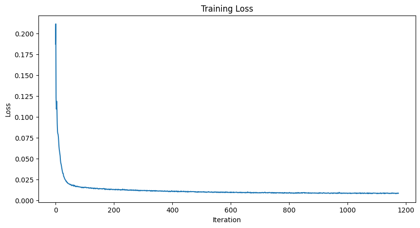
Training Loss Curve
To iteratively denoise an image from pure noise, the UNet can be conditioned on a time variable. Then, following the two algorithms from the DDPM paper, we can train our model to iteratively denoise pure noise to ground truth images, and then run inference by following the sampling algorthm. Here is the training curve as well as results for generation from pure noise from training the model after the 5th and 20th epoch.


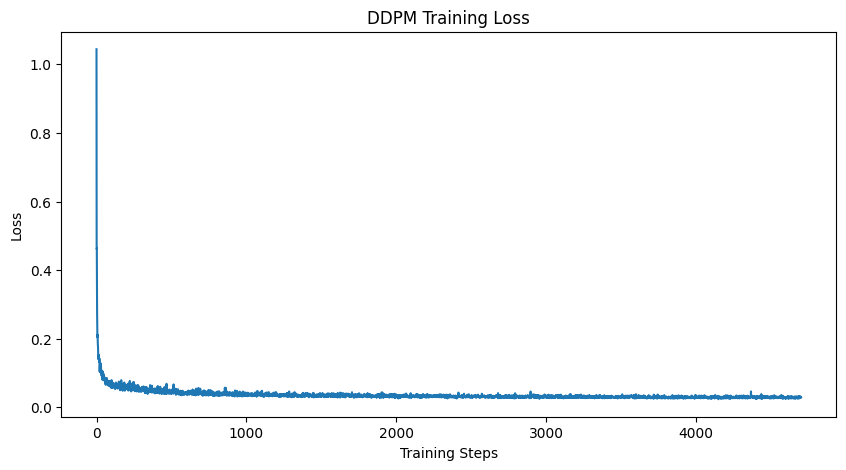 Training Loss Curve

Epoch 5

Epoch 20
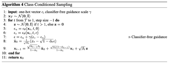
By incoporating a class condition into the UNet which is retrieved from the labels in the dataset, we can manually set which number from 0 to 9 that should be generated. On top of this, at sampling time, classifier-free guidance is implemented to help create better generations by following algorithm 4 from the DDPM paper.
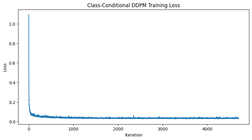
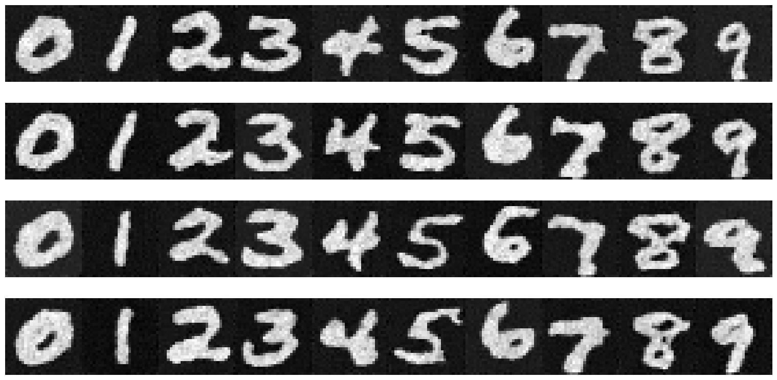
Epoch 5 Results
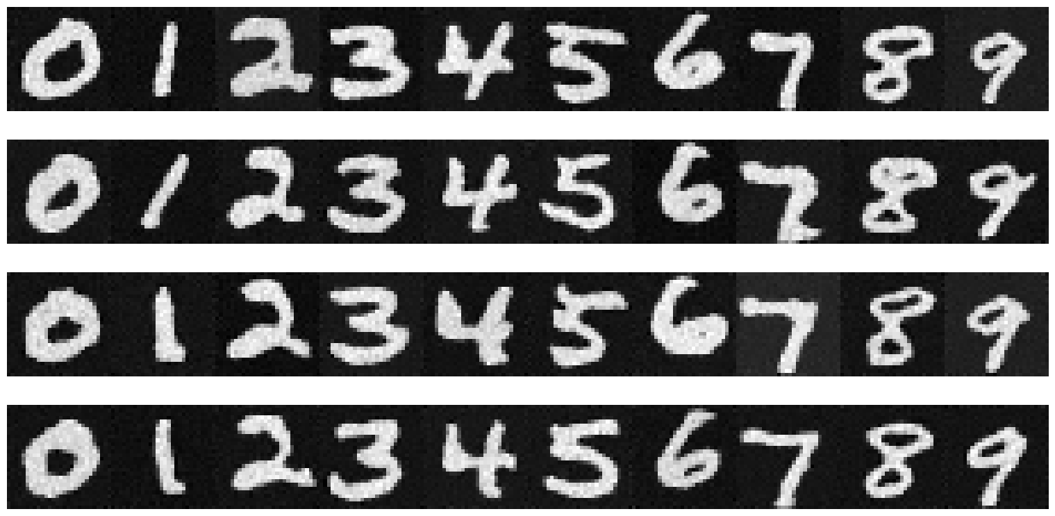
Epoch 20 Results
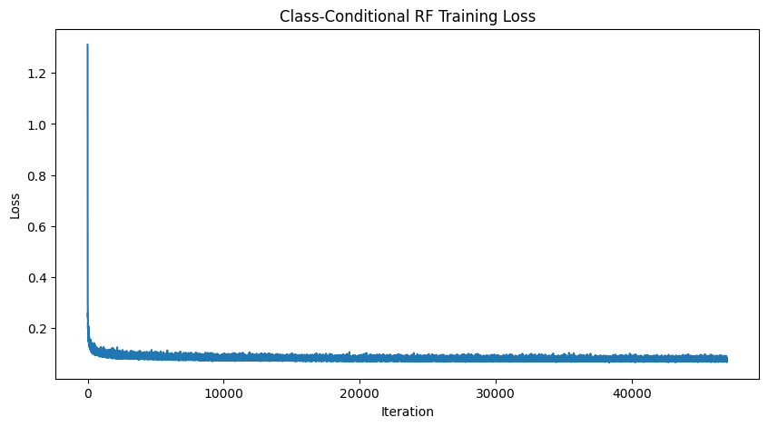
Rectified flow is another paradigm for generative modeling based on flow matching. The main difference between rectified flow (RF) and diffusion is that RF is a transport problem, while diffusion is a denoising task. RF learns to map one distribution to another. In our case for MNIST digit generation, RF learns to transport the gaussian distribution to the distribution of MNIST. Rather than noise an image and learn to denoise it, we can start with samples from gaussian noise and learn to transport it to MNIST. Rectified flow trajectories are also linear, meaning that when we do sampling for training, for any given timestep t, we can simply linearly interpolate between the ground turth and the noise sample to get the true ground truth of the image at that timestep.
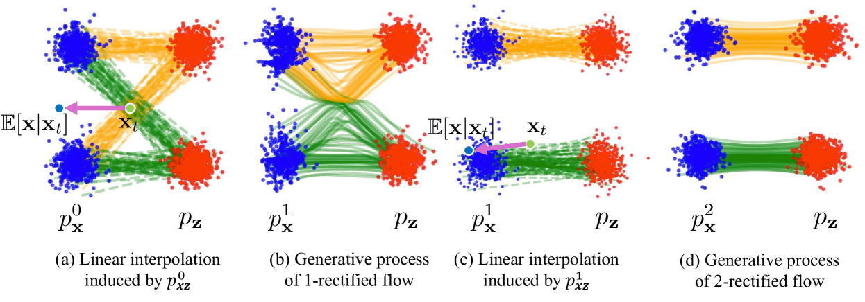
Rectified Flow
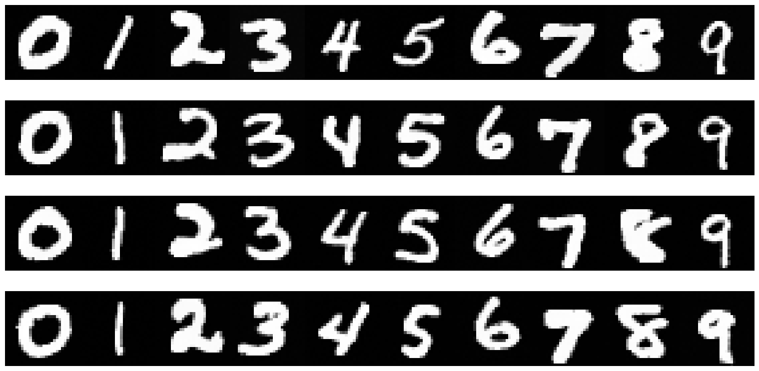
RF Generated Images